Session 6: Neural Networks

This course is interesting because it brings together two incredibly complex and rapidly-advancing topics: digital design and machine learning. Now that we’ve wrapped our heads around a few core concepts in the former space, we’re ready to see how to apply our skills to a novel scenario.

Let’s first remind ourselves of our goal: building an inference accelerator on an FPGA. But what exactly are we going to accelerate?

Deep learning

Deep learning is subcategory in the domain of machine learning, which is itself a subcategory of the field of artificial intelligence. It gains its name from the fact that information travels several layers deep through an arrangement of so-called neurons. It is simply one of many approaches to AI but it is also one that has received tremendous attention in the past decade, in part due to its excellent accuracy.

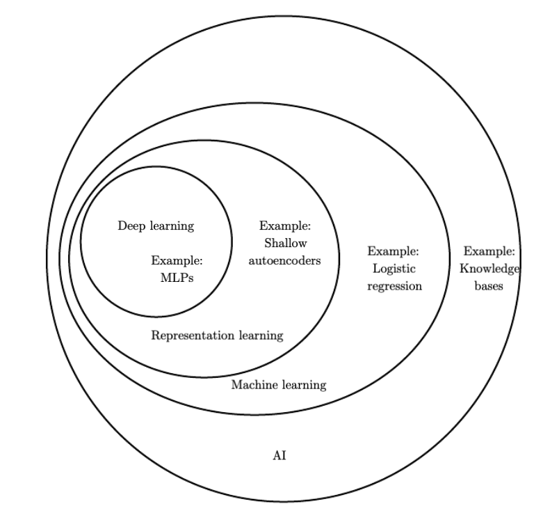
*Figure taken from https://www.deeplearningbook.org/contents/intro.html

Network topologies

The quintessential example of a deep learning model is the feedforward deep network, or multilayer perceptron (MLP). This is also called a fully connected network.

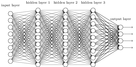
*Figure taken from http://neuralnetworksanddeeplearning.com

A few observations:

• Information travels from left to right
• All neurons in one layer are connected to all neurons in the next
• There is one input and one output layer as well several intermediate “hidden” layers

Another kind of neural network is a convolutional network. We’re going to be building one of these. They’re known for their high accuracy with image inputs due to their awareness of spatial features.

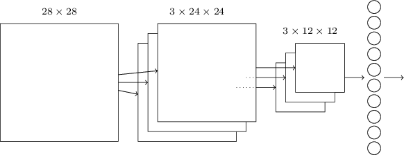
*Figure taken from http://neuralnetworksanddeeplearning.com

The basic structure is as follows:

1. Information resident in the 28x28 grid gets gradually reduced to the last output layer with 10 neurons.
2. The middle layer is called the convolutional layer and is formed of several feature maps.
3. Each feature map is then turned into a unit in the pooling layer.
4. Finally, all neurons in the pooling layer are connected to all 10 neurons in the output layer, reminiscent of our fully-connected network.

The ‘convolution’ in the name comes from the fact that the initial operation applied to the image to obtain the feature maps is known as a convolution.

Note

We could, of course, train an MLP and use it for inference. For our relatively well-scoped problem of digit recognition on a 28x28 grid of greyscale pixels, both approaches would work well. That said, MLPs are considered ‘old technology’, having been around for decades before CNNs and are rarely used for image recognition. CNNs themselves were introduced in a seminal paper by LeCun and others in 1998!

Training and inference

Machine learning is a two-step process.

Tip

I’ve found that neural networks can be somewhat of a misnomer. You can draw an equivalence between human neurons firing and being interconnected in a complex web but that’s pretty much where the analogy stops. I’d therefore encourage you to think more in terms of ‘nodes’ or ‘units’ and as the whole system being just a function.